7. Finetuning for Text Classification

from importlib.metadata import version

pkgs = ["matplotlib",
        "numpy",
        "tiktoken",
        "torch",
        "tensorflow", # For OpenAI's pretrained weights
        "pandas"      # Dataset loading
       ]
for p in pkgs:
    print(f"{p} version: {version(p)}")

matplotlib version: 3.8.2
numpy version: 1.26.0
tiktoken version: 0.5.1
torch version: 2.2.2
tensorflow version: 2.15.0
pandas version: 2.2.1

7.1. Different categories of finetuning

• No code in this section

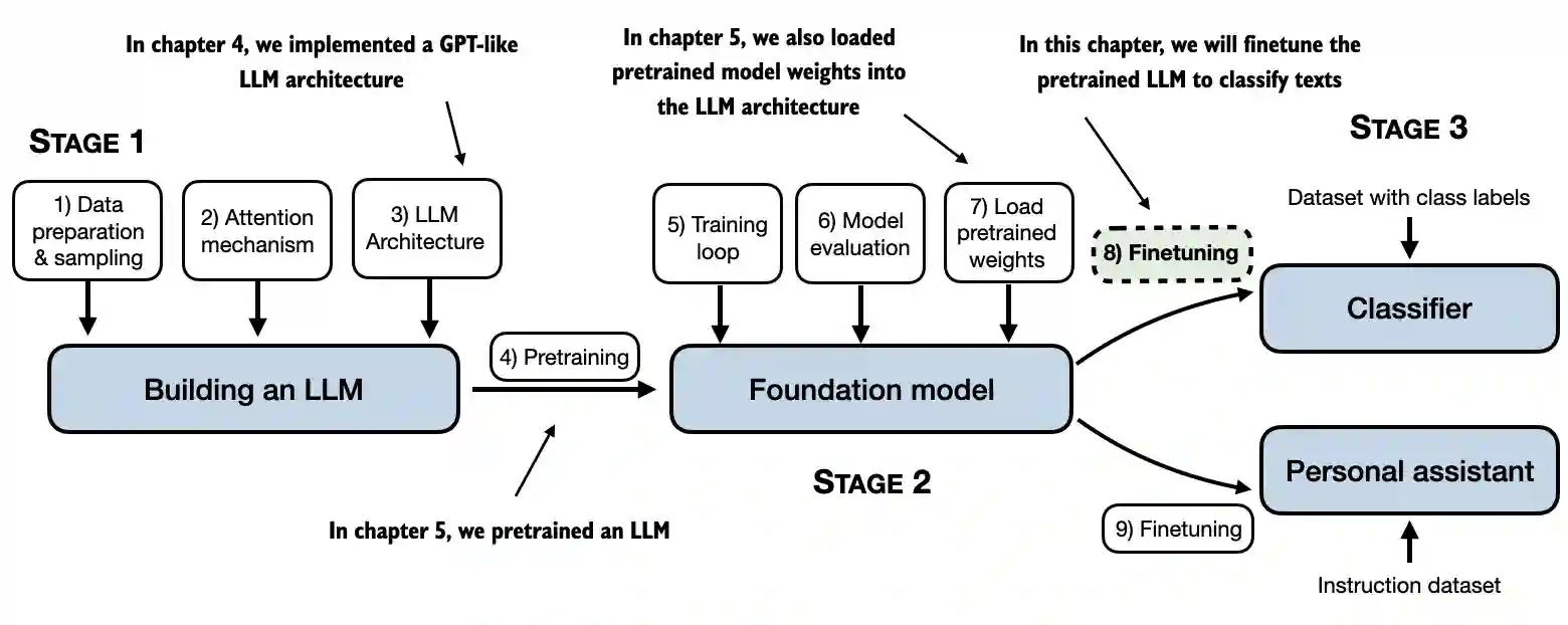
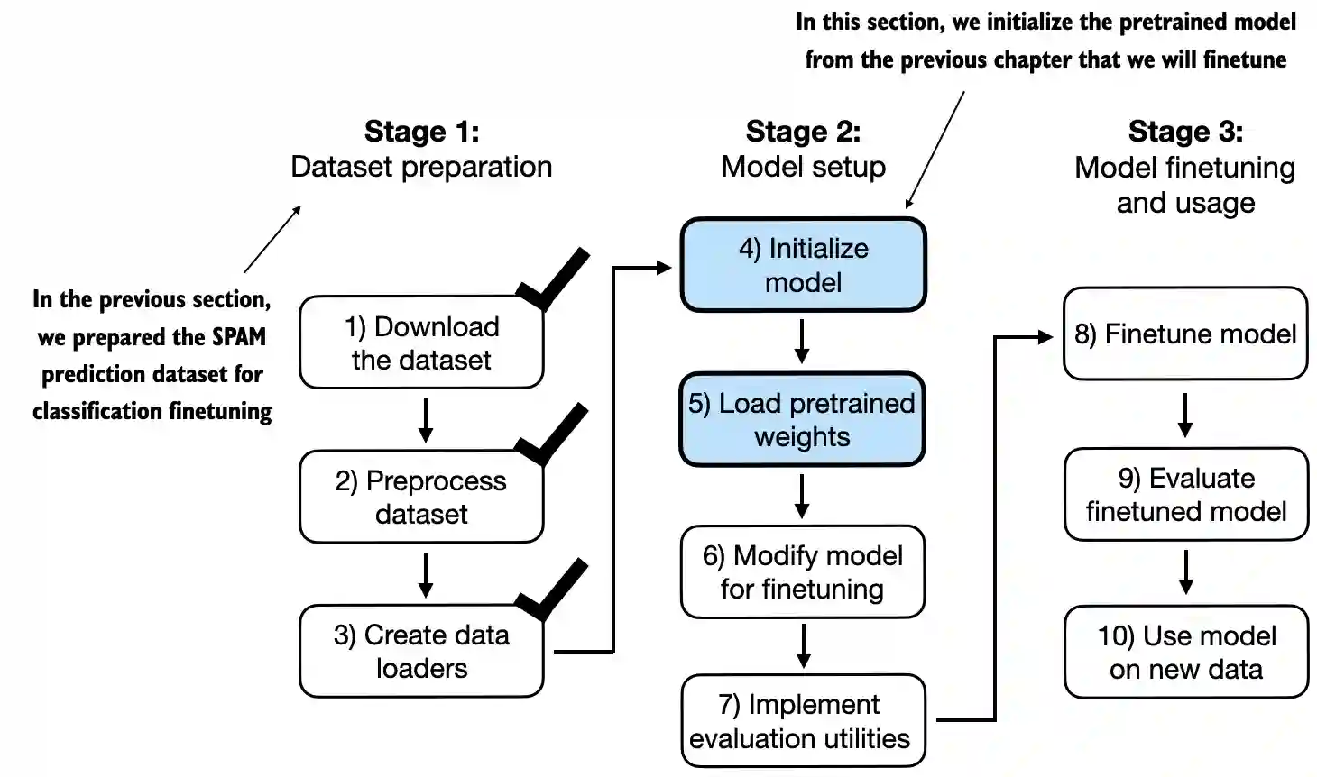
• The most common ways to finetune language models are instruction-finetuning and classification finetuning

• Instruction-finetuning, depicted below, is the topic of the next chapter

• Classification finetuning, the topic of this chapter, is a procedure you may already be familiar with if you have a background in machine learning – it’s similar to training a convolutional network to classify handwritten digits, for example

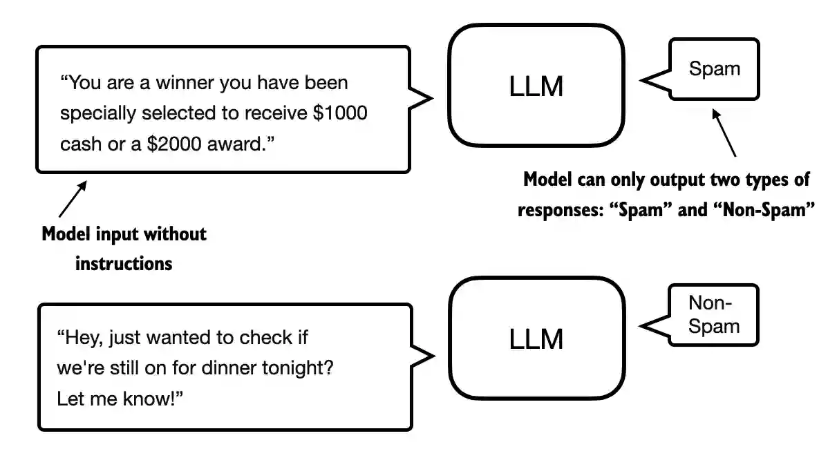
• In classification finetuning, we have a specific number of class labels (for example, “spam” and “not spam”) that the model can output

• A classification finetuned model can only predict classes it has seen during training (for example, “spam” or “not spam”, whereas an instruction-finetuned model can usually perform many tasks

• We can think of a classification-finetuned model as a very specialized model; in practice, it is much easier to create a specialized model than a generalist model that performs well on many different tasks

7.2. Preparing the dataset

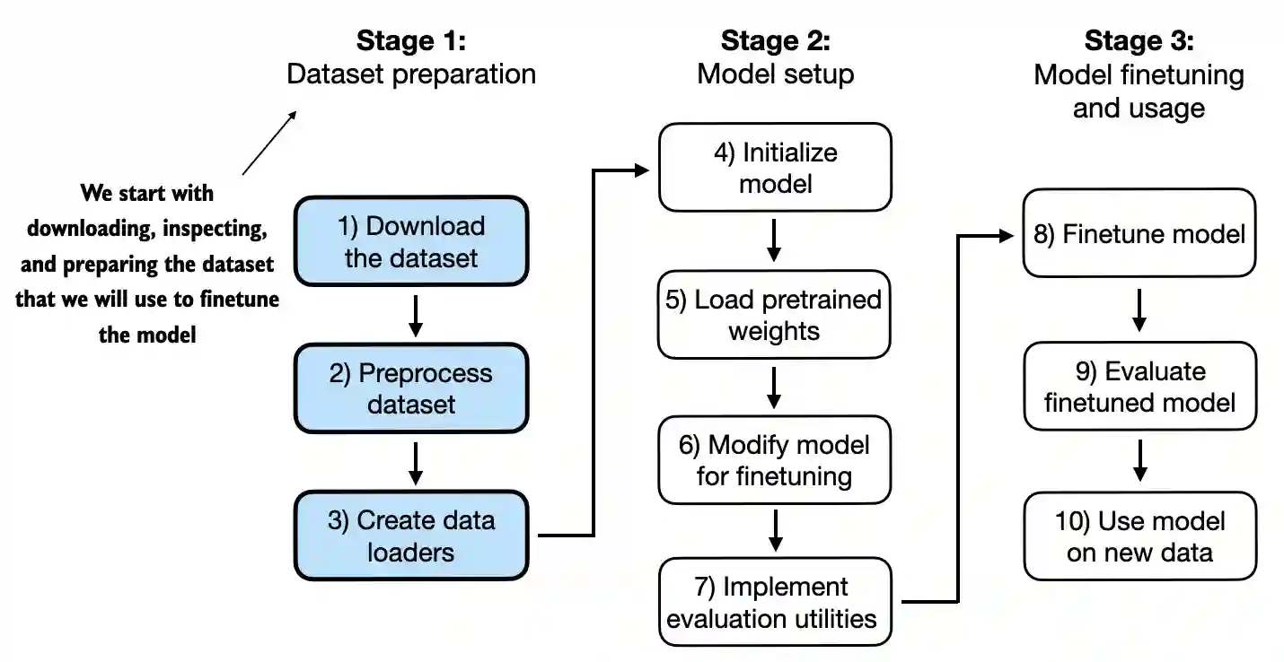
• This section prepares the dataset we use for classification finetuning

• We use a dataset consisting of spam and non-spam text messages to finetune the LLM to classify them

• First, we download and unzip the dataset

import urllib.request
import zipfile
import os
from pathlib import Path

url = "https://archive.ics.uci.edu/static/public/228/sms+spam+collection.zip"
zip_path = "sms_spam_collection.zip"
extracted_path = "sms_spam_collection"
data_file_path = Path(extracted_path) / "SMSSpamCollection.tsv"

def download_and_unzip(url, zip_path, extracted_path, data_file_path):
    if data_file_path.exists():
        print(f"{data_file_path} already exists. Skipping download and extraction.")
        return

    # Downloading the file
    with urllib.request.urlopen(url) as response:
        with open(zip_path, "wb") as out_file:
            out_file.write(response.read())

    # Unzipping the file
    with zipfile.ZipFile(zip_path, "r") as zip_ref:
        zip_ref.extractall(extracted_path)

    # Add .tsv file extension
    original_file_path = Path(extracted_path) / "SMSSpamCollection"
    os.rename(original_file_path, data_file_path)
    print(f"File downloaded and saved as {data_file_path}")

download_and_unzip(url, zip_path, extracted_path, data_file_path)

sms_spam_collection/SMSSpamCollection.tsv already exists. Skipping download and extraction.

• The dataset is saved as a tab-separated text file, which we can load into a pandas DataFrame

import pandas as pd

df = pd.read_csv(data_file_path, sep="\t", header=None, names=["Label", "Text"])
df

	Label	Text
0	ham	Go until jurong point, crazy.. Available only ...
1	ham	Ok lar... Joking wif u oni...
2	spam	Free entry in 2 a wkly comp to win FA Cup fina...
3	ham	U dun say so early hor... U c already then say...
4	ham	Nah I don't think he goes to usf, he lives aro...
...	...	...
5567	spam	This is the 2nd time we have tried 2 contact u...
5568	ham	Will ü b going to esplanade fr home?
5569	ham	Pity, * was in mood for that. So...any other s...
5570	ham	The guy did some bitching but I acted like i'd...
5571	ham	Rofl. Its true to its name

5572 rows × 2 columns

• When we check the class distribution, we see that the data contains “ham” (i.e., “not spam”) much more frequently than “spam”

print(df["Label"].value_counts())

Label
ham     4825
spam     747
Name: count, dtype: int64

• For simplicity, and because we prefer a small dataset for educational purposes anyway (it will make it possible to finetune the LLM faster), we subsample (undersample) the dataset so that it contains 747 instances from each class

• (Next to undersampling, there are several other ways to deal with class balances, but they are out of the scope of a book on LLMs; you can find examples and more information in the imbalanced-learn user guide)

def create_balanced_dataset(df):
    
    # Count the instances of "spam"
    num_spam = df[df["Label"] == "spam"].shape[0]
    
    # Randomly sample "ham" instances to match the number of "spam" instances
    ham_subset = df[df["Label"] == "ham"].sample(num_spam, random_state=123)
    
    # Combine ham "subset" with "spam"
    balanced_df = pd.concat([ham_subset, df[df["Label"] == "spam"]])

    return balanced_df

balanced_df = create_balanced_dataset(df)
print(balanced_df["Label"].value_counts())

Label
ham     747
spam    747
Name: count, dtype: int64

• Next, we change the string class labels “ham” and “spam” into integer class labels 0 and 1:

balanced_df["Label"] = balanced_df["Label"].map({"ham": 0, "spam": 1})

• Let’s now define a function that randomly divides the dataset into a training, validation, and test subset

def random_split(df, train_frac, validation_frac):
    # Shuffle the entire DataFrame
    df = df.sample(frac=1, random_state=123).reset_index(drop=True)

    # Calculate split indices
    train_end = int(len(df) * train_frac)
    validation_end = train_end + int(len(df) * validation_frac)

    # Split the DataFrame
    train_df = df[:train_end]
    validation_df = df[train_end:validation_end]
    test_df = df[validation_end:]

    return train_df, validation_df, test_df

train_df, validation_df, test_df = random_split(balanced_df, 0.7, 0.1)
# Test size is implied to be 0.2 as the remainder

train_df.to_csv("train.csv", index=None)
validation_df.to_csv("validation.csv", index=None)
test_df.to_csv("test.csv", index=None)

7.3. Creating data loaders

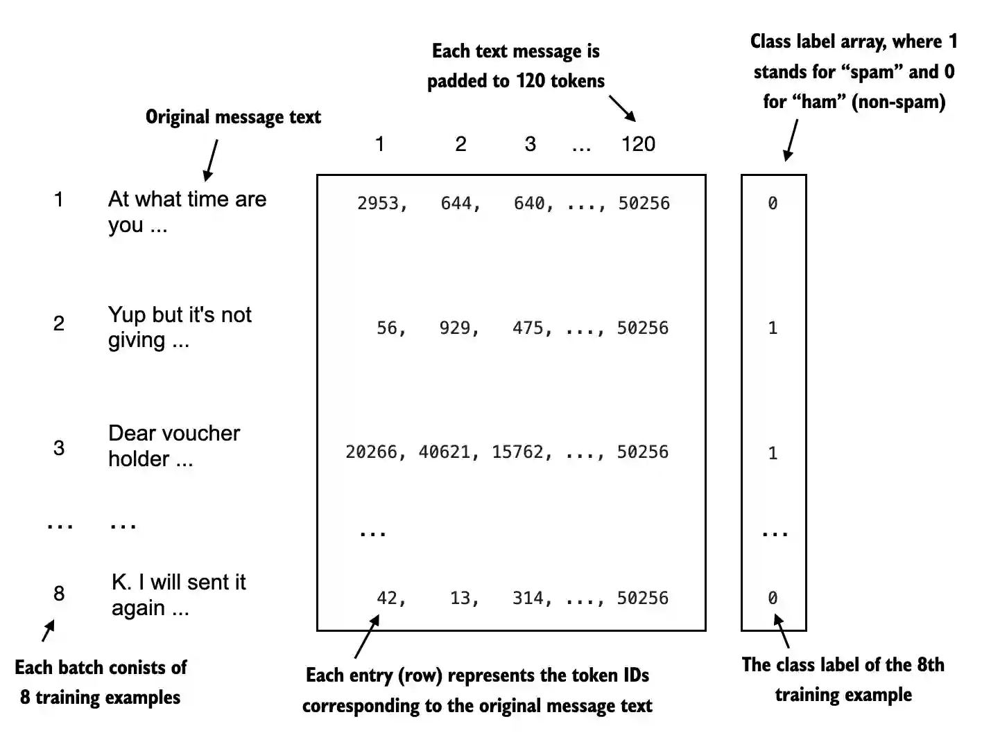
• Note that the text messages have different lengths; if we want to combine multiple training examples in a batch, we have to either

  • 1. truncate all messages to the length of the shortest message in the dataset or batch

  • 1. pad all messages to the length of the longest message in the dataset or batch

• We choose option 2 and pad all messages to the longest message in the dataset

• For that, we use <|endoftext|> as a padding token, as discussed in chapter 2

import tiktoken

tokenizer = tiktoken.get_encoding("gpt2")
print(tokenizer.encode("<|endoftext|>", allowed_special={"<|endoftext|>"}))

[50256]

token_ids = tokenizer.encode("This is the first text message")
print(token_ids)

[1212, 318, 262, 717, 2420, 3275]

• The SpamDataset class below identifies the longest sequence in the training dataset and adds the padding token to the others to match that sequence length

import torch
from torch.utils.data import Dataset


class SpamDataset(Dataset):
    def __init__(self, csv_file, tokenizer, max_length=None, pad_token_id=50256):
        self.data = pd.read_csv(csv_file)

        # Pre-tokenize texts
        self.encoded_texts = [
            tokenizer.encode(text) for text in self.data["Text"]
        ]

        if max_length is None:
            self.max_length = self._longest_encoded_length()
        else:
            self.max_length = max_length
            # Truncate sequences if they are longer than max_length
            self.encoded_texts = [
                encoded_text[:self.max_length]
                for encoded_text in self.encoded_texts
            ]

        # Pad sequences to the longest sequence
        self.encoded_texts = [
            encoded_text + [pad_token_id] * (self.max_length - len(encoded_text))
            for encoded_text in self.encoded_texts
        ]

    def __getitem__(self, index):
        encoded = self.encoded_texts[index]
        label = self.data.iloc[index]["Label"]
        return (
            torch.tensor(encoded, dtype=torch.long),
            torch.tensor(label, dtype=torch.long)
        )

    def __len__(self):
        return len(self.data)

    def _longest_encoded_length(self):
        max_length = 0
        for encoded_text in self.encoded_texts:
            encoded_length = len(encoded_text)
            if encoded_length > max_length:
                max_length = encoded_length
        return max_length

train_dataset = SpamDataset(
    csv_file="train.csv",
    max_length=None,
    tokenizer=tokenizer
)

print(train_dataset.max_length)

120

• We also pad the validation and test set to the longest training sequence

• Note that validation and test set samples that are longer than the longest training example are being truncated via encoded_text[:self.max_length] in the SpamDataset code

• This behavior is entirely optional, and it would also work well if we set max_length=None in both the validation and test set cases

val_dataset = SpamDataset(
    csv_file="validation.csv",
    max_length=train_dataset.max_length,
    tokenizer=tokenizer
)
test_dataset = SpamDataset(
    csv_file="test.csv",
    max_length=train_dataset.max_length,
    tokenizer=tokenizer
)

• Next, we use the dataset to instantiate the data loaders, which is similar to creating the data loaders in previous chapters

from torch.utils.data import DataLoader

num_workers = 0
batch_size = 8

torch.manual_seed(123)

train_loader = DataLoader(
    dataset=train_dataset,
    batch_size=batch_size,
    shuffle=True,
    num_workers=num_workers,
    drop_last=True,
)

val_loader = DataLoader(
    dataset=val_dataset,
    batch_size=batch_size,
    num_workers=num_workers,
    drop_last=False,
)

test_loader = DataLoader(
    dataset=test_dataset,
    batch_size=batch_size,
    num_workers=num_workers,
    drop_last=False,
)

• As a verification step, we iterate through the data loaders and ensure that the batches contain 8 training examples each, where each training example consists of 120 tokens

print("Train loader:")
for input_batch, target_batch in train_loader:
    pass

print("Input batch dimensions:", input_batch.shape)
print("Label batch dimensions", target_batch.shape)

Train loader:
Input batch dimensions: torch.Size([8, 120])
Label batch dimensions torch.Size([8])

• Lastly, let’s print the total number of batches in each dataset

print(f"{len(train_loader)} training batches")
print(f"{len(val_loader)} validation batches")
print(f"{len(test_loader)} test batches")

130 training batches
19 validation batches
38 test batches

7.4. Initializing a model with pretrained weights

• In this section, we initialize the pretrained model we worked with in the previous chapter

CHOOSE_MODEL = "gpt2-small (124M)"
INPUT_PROMPT = "Every effort moves"

BASE_CONFIG = {
    "vocab_size": 50257,     # Vocabulary size
    "context_length": 1024,  # Context length
    "drop_rate": 0.0,        # Dropout rate
    "qkv_bias": True         # Query-key-value bias
}

model_configs = {
    "gpt2-small (124M)": {"emb_dim": 768, "n_layers": 12, "n_heads": 12},
    "gpt2-medium (355M)": {"emb_dim": 1024, "n_layers": 24, "n_heads": 16},
    "gpt2-large (774M)": {"emb_dim": 1280, "n_layers": 36, "n_heads": 20},
    "gpt2-xl (1558M)": {"emb_dim": 1600, "n_layers": 48, "n_heads": 25},
}

BASE_CONFIG.update(model_configs[CHOOSE_MODEL])

from gpt_download import download_and_load_gpt2
from previous_chapters import GPTModel, load_weights_into_gpt

model_size = CHOOSE_MODEL.split(" ")[-1].lstrip("(").rstrip(")")
settings, params = download_and_load_gpt2(model_size=model_size, models_dir="gpt2")

model = GPTModel(BASE_CONFIG)
load_weights_into_gpt(model, params)
model.eval();

checkpoint: 100%|███████████████████████████| 77.0/77.0 [00:00<00:00, 39.7kiB/s]
encoder.json: 100%|███████████████████████| 1.04M/1.04M [00:00<00:00, 3.25MiB/s]
hparams.json: 100%|█████████████████████████| 90.0/90.0 [00:00<00:00, 51.4kiB/s]
model.ckpt.data-00000-of-00001: 100%|███████| 498M/498M [01:00<00:00, 8.20MiB/s]
model.ckpt.index: 100%|███████████████████| 5.21k/5.21k [00:00<00:00, 2.34MiB/s]
model.ckpt.meta: 100%|██████████████████████| 471k/471k [00:00<00:00, 2.26MiB/s]
vocab.bpe: 100%|████████████████████████████| 456k/456k [00:00<00:00, 2.62MiB/s]

• To ensure that the model was loaded corrected, let’s double-check that it generates coherent text

from previous_chapters import (
    generate_text_simple,
    text_to_token_ids,
    token_ids_to_text
)


text_1 = "Every effort moves you"

token_ids = generate_text_simple(
    model=model,
    idx=text_to_token_ids(text_1, tokenizer),
    max_new_tokens=15,
    context_size=BASE_CONFIG["context_length"]
)

print(token_ids_to_text(token_ids, tokenizer))

Every effort moves you forward.

The first step is to understand the importance of your work

• Before we finetune the model as a classifier, let’s see if the model can perhaps already classify spam messages via prompting

text_2 = (
    "Is the following text 'spam'? Answer with 'yes' or 'no':"
    " 'You are a winner you have been specially"
    " selected to receive $1000 cash or a $2000 award.'"
    " Answer with 'yes' or 'no'."
)

token_ids = generate_text_simple(
    model=model,
    idx=text_to_token_ids(text_2, tokenizer),
    max_new_tokens=23,
    context_size=BASE_CONFIG["context_length"]
)

print(token_ids_to_text(token_ids, tokenizer))

Is the following text 'spam'? Answer with 'yes' or 'no': 'You are a winner you have been specially selected to receive $1000 cash or a $2000 award.' Answer with 'yes' or 'no'. Answer with 'yes' or 'no'. Answer with 'yes' or 'no'. Answer with 'yes'

• As we can see, the model is not very good at following instruction

• This is expected, since it has only been pretrained and not instruction-finetuned (instruction finetuning will be covered in the next chapter)

7.5. Adding a classification head

• In this section, we are modifying the pretrained LLM to make it ready for classification finetuning

• Let’s take a look at the model architecture first

print(model)

GPTModel(
  (tok_emb): Embedding(50257, 768)
  (pos_emb): Embedding(1024, 768)
  (drop_emb): Dropout(p=0.0, inplace=False)
  (trf_blocks): Sequential(
    (0): TransformerBlock(
      (att): MultiHeadAttention(
        (W_query): Linear(in_features=768, out_features=768, bias=True)
        (W_key): Linear(in_features=768, out_features=768, bias=True)
        (W_value): Linear(in_features=768, out_features=768, bias=True)
        (out_proj): Linear(in_features=768, out_features=768, bias=True)
        (dropout): Dropout(p=0.0, inplace=False)
      )
      (ff): FeedForward(
        (layers): Sequential(
          (0): Linear(in_features=768, out_features=3072, bias=True)
          (1): GELU()
          (2): Linear(in_features=3072, out_features=768, bias=True)
        )
      )
      (norm1): LayerNorm()
      (norm2): LayerNorm()
      (drop_resid): Dropout(p=0.0, inplace=False)
    )
    (1): TransformerBlock(
      (att): MultiHeadAttention(
        (W_query): Linear(in_features=768, out_features=768, bias=True)
        (W_key): Linear(in_features=768, out_features=768, bias=True)
        (W_value): Linear(in_features=768, out_features=768, bias=True)
        (out_proj): Linear(in_features=768, out_features=768, bias=True)
        (dropout): Dropout(p=0.0, inplace=False)
      )
      (ff): FeedForward(
        (layers): Sequential(
          (0): Linear(in_features=768, out_features=3072, bias=True)
          (1): GELU()
          (2): Linear(in_features=3072, out_features=768, bias=True)
        )
      )
      (norm1): LayerNorm()
      (norm2): LayerNorm()
      (drop_resid): Dropout(p=0.0, inplace=False)
    )
    (2): TransformerBlock(
      (att): MultiHeadAttention(
        (W_query): Linear(in_features=768, out_features=768, bias=True)
        (W_key): Linear(in_features=768, out_features=768, bias=True)
        (W_value): Linear(in_features=768, out_features=768, bias=True)
        (out_proj): Linear(in_features=768, out_features=768, bias=True)
        (dropout): Dropout(p=0.0, inplace=False)
      )
      (ff): FeedForward(
        (layers): Sequential(
          (0): Linear(in_features=768, out_features=3072, bias=True)
          (1): GELU()
          (2): Linear(in_features=3072, out_features=768, bias=True)
        )
      )
      (norm1): LayerNorm()
      (norm2): LayerNorm()
      (drop_resid): Dropout(p=0.0, inplace=False)
    )
    (3): TransformerBlock(
      (att): MultiHeadAttention(
        (W_query): Linear(in_features=768, out_features=768, bias=True)
        (W_key): Linear(in_features=768, out_features=768, bias=True)
        (W_value): Linear(in_features=768, out_features=768, bias=True)
        (out_proj): Linear(in_features=768, out_features=768, bias=True)
        (dropout): Dropout(p=0.0, inplace=False)
      )
      (ff): FeedForward(
        (layers): Sequential(
          (0): Linear(in_features=768, out_features=3072, bias=True)
          (1): GELU()
          (2): Linear(in_features=3072, out_features=768, bias=True)
        )
      )
      (norm1): LayerNorm()
      (norm2): LayerNorm()
      (drop_resid): Dropout(p=0.0, inplace=False)
    )
    (4): TransformerBlock(
      (att): MultiHeadAttention(
        (W_query): Linear(in_features=768, out_features=768, bias=True)
        (W_key): Linear(in_features=768, out_features=768, bias=True)
        (W_value): Linear(in_features=768, out_features=768, bias=True)
        (out_proj): Linear(in_features=768, out_features=768, bias=True)
        (dropout): Dropout(p=0.0, inplace=False)
      )
      (ff): FeedForward(
        (layers): Sequential(
          (0): Linear(in_features=768, out_features=3072, bias=True)
          (1): GELU()
          (2): Linear(in_features=3072, out_features=768, bias=True)
        )
      )
      (norm1): LayerNorm()
      (norm2): LayerNorm()
      (drop_resid): Dropout(p=0.0, inplace=False)
    )
    (5): TransformerBlock(
      (att): MultiHeadAttention(
        (W_query): Linear(in_features=768, out_features=768, bias=True)
        (W_key): Linear(in_features=768, out_features=768, bias=True)
        (W_value): Linear(in_features=768, out_features=768, bias=True)
        (out_proj): Linear(in_features=768, out_features=768, bias=True)
        (dropout): Dropout(p=0.0, inplace=False)
      )
      (ff): FeedForward(
        (layers): Sequential(
          (0): Linear(in_features=768, out_features=3072, bias=True)
          (1): GELU()
          (2): Linear(in_features=3072, out_features=768, bias=True)
        )
      )
      (norm1): LayerNorm()
      (norm2): LayerNorm()
      (drop_resid): Dropout(p=0.0, inplace=False)
    )
    (6): TransformerBlock(
      (att): MultiHeadAttention(
        (W_query): Linear(in_features=768, out_features=768, bias=True)
        (W_key): Linear(in_features=768, out_features=768, bias=True)
        (W_value): Linear(in_features=768, out_features=768, bias=True)
        (out_proj): Linear(in_features=768, out_features=768, bias=True)
        (dropout): Dropout(p=0.0, inplace=False)
      )
      (ff): FeedForward(
        (layers): Sequential(
          (0): Linear(in_features=768, out_features=3072, bias=True)
          (1): GELU()
          (2): Linear(in_features=3072, out_features=768, bias=True)
        )
      )
      (norm1): LayerNorm()
      (norm2): LayerNorm()
      (drop_resid): Dropout(p=0.0, inplace=False)
    )
    (7): TransformerBlock(
      (att): MultiHeadAttention(
        (W_query): Linear(in_features=768, out_features=768, bias=True)
        (W_key): Linear(in_features=768, out_features=768, bias=True)
        (W_value): Linear(in_features=768, out_features=768, bias=True)
        (out_proj): Linear(in_features=768, out_features=768, bias=True)
        (dropout): Dropout(p=0.0, inplace=False)
      )
      (ff): FeedForward(
        (layers): Sequential(
          (0): Linear(in_features=768, out_features=3072, bias=True)
          (1): GELU()
          (2): Linear(in_features=3072, out_features=768, bias=True)
        )
      )
      (norm1): LayerNorm()
      (norm2): LayerNorm()
      (drop_resid): Dropout(p=0.0, inplace=False)
    )
    (8): TransformerBlock(
      (att): MultiHeadAttention(
        (W_query): Linear(in_features=768, out_features=768, bias=True)
        (W_key): Linear(in_features=768, out_features=768, bias=True)
        (W_value): Linear(in_features=768, out_features=768, bias=True)
        (out_proj): Linear(in_features=768, out_features=768, bias=True)
        (dropout): Dropout(p=0.0, inplace=False)
      )
      (ff): FeedForward(
        (layers): Sequential(
          (0): Linear(in_features=768, out_features=3072, bias=True)
          (1): GELU()
          (2): Linear(in_features=3072, out_features=768, bias=True)
        )
      )
      (norm1): LayerNorm()
      (norm2): LayerNorm()
      (drop_resid): Dropout(p=0.0, inplace=False)
    )
    (9): TransformerBlock(
      (att): MultiHeadAttention(
        (W_query): Linear(in_features=768, out_features=768, bias=True)
        (W_key): Linear(in_features=768, out_features=768, bias=True)
        (W_value): Linear(in_features=768, out_features=768, bias=True)
        (out_proj): Linear(in_features=768, out_features=768, bias=True)
        (dropout): Dropout(p=0.0, inplace=False)
      )
      (ff): FeedForward(
        (layers): Sequential(
          (0): Linear(in_features=768, out_features=3072, bias=True)
          (1): GELU()
          (2): Linear(in_features=3072, out_features=768, bias=True)
        )
      )
      (norm1): LayerNorm()
      (norm2): LayerNorm()
      (drop_resid): Dropout(p=0.0, inplace=False)
    )
    (10): TransformerBlock(
      (att): MultiHeadAttention(
        (W_query): Linear(in_features=768, out_features=768, bias=True)
        (W_key): Linear(in_features=768, out_features=768, bias=True)
        (W_value): Linear(in_features=768, out_features=768, bias=True)
        (out_proj): Linear(in_features=768, out_features=768, bias=True)
        (dropout): Dropout(p=0.0, inplace=False)
      )
      (ff): FeedForward(
        (layers): Sequential(
          (0): Linear(in_features=768, out_features=3072, bias=True)
          (1): GELU()
          (2): Linear(in_features=3072, out_features=768, bias=True)
        )
      )
      (norm1): LayerNorm()
      (norm2): LayerNorm()
      (drop_resid): Dropout(p=0.0, inplace=False)
    )
    (11): TransformerBlock(
      (att): MultiHeadAttention(
        (W_query): Linear(in_features=768, out_features=768, bias=True)
        (W_key): Linear(in_features=768, out_features=768, bias=True)
        (W_value): Linear(in_features=768, out_features=768, bias=True)
        (out_proj): Linear(in_features=768, out_features=768, bias=True)
        (dropout): Dropout(p=0.0, inplace=False)
      )
      (ff): FeedForward(
        (layers): Sequential(
          (0): Linear(in_features=768, out_features=3072, bias=True)
          (1): GELU()
          (2): Linear(in_features=3072, out_features=768, bias=True)
        )
      )
      (norm1): LayerNorm()
      (norm2): LayerNorm()
      (drop_resid): Dropout(p=0.0, inplace=False)
    )
  )
  (final_norm): LayerNorm()
  (out_head): Linear(in_features=768, out_features=50257, bias=False)
)

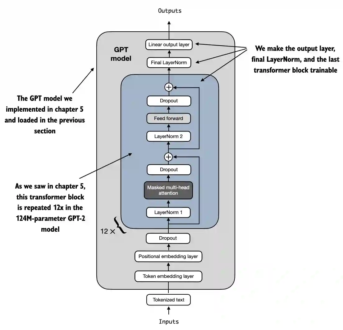
• Above, we can see the architecture we implemented in chapter 4 neatly laid out

• The goal is to replace and finetune the output layer

• To achieve this, we first freeze the model, meaning that we make all layers non-trainable

for param in model.parameters():
    param.requires_grad = False

• Then, we replace the output layer (model.out_head), which originally maps the layer inputs to 50,257 dimensions (the size of the vocabulary)

• Since we finetune the model for binary classification (predicting 2 classes, “spam” and “not spam”), we can replace the output layer as shown below, which will be trainable by default

• Note that we use BASE_CONFIG["emb_dim"] (which is equal to 768 in the "gpt2-small (124M)" model) to keep the code below more general

torch.manual_seed(123)

num_classes = 2
model.out_head = torch.nn.Linear(in_features=BASE_CONFIG["emb_dim"], out_features=num_classes)

• Technically, it’s sufficient to only train the output layer

• However, as I found in experiments finetuning additional layers can noticeably improve the performance

• So, we are also making the last transformer block and the final LayerNorm module connecting the last transformer block to the output layer trainable

for param in model.trf_blocks[-1].parameters():
    param.requires_grad = True

for param in model.final_norm.parameters():
    param.requires_grad = True

• We can still use this model similar to before in previous chapters

• For example, let’s feed it some text input

inputs = tokenizer.encode("Do you have time")
inputs = torch.tensor(inputs).unsqueeze(0)
print("Inputs:", inputs)
print("Inputs dimensions:", inputs.shape) # shape: (batch_size, num_tokens)

Inputs: tensor([[5211,  345,  423,  640]])
Inputs dimensions: torch.Size([1, 4])

• What’s different compared to previous chapters is that it now has two output dimensions instead of 50,257

with torch.no_grad():
    outputs = model(inputs)

print("Outputs:\n", outputs)
print("Outputs dimensions:", outputs.shape) # shape: (batch_size, num_tokens, num_classes)

Outputs:
 tensor([[[-1.5854,  0.9904],
         [-3.7235,  7.4548],
         [-2.2661,  6.6049],
         [-3.5983,  3.9902]]])
Outputs dimensions: torch.Size([1, 4, 2])

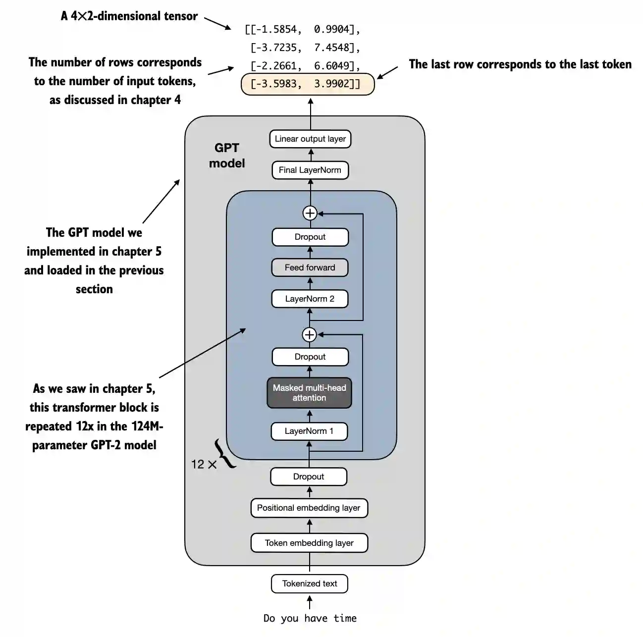
• As discussed in previous chapters, for each input token, there’s one output vector

• Since we fed the model a text sample with 6 input tokens, the output consists of 6 2-dimensional output vectors above

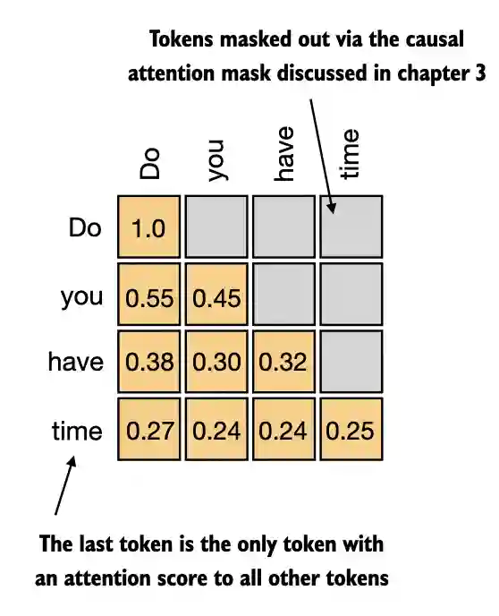
• In chapter 3, we discussed the attention mechanism, which connects each input token to each other input token

• In chapter 3, we then also introduced the causal attention mask that is used in GPT-like models; this causal mask lets a current token only attend to the current and previous token positions

• Based on this causal attention mechanism, the 6th (last) token above contains the most information among all tokens because it’s the only token that includes information about all other tokens

• Hence, we are particularly interested in this last token, which we will finetune for the spam classification task

print("Last output token:", outputs[:, -1, :])

Last output token: tensor([[-5.7543,  5.3615]])

7.6. Calculating the classification loss and accuracy

• Before we can start finetuning (/training), we first have to define the loss function we want to optimize during training

• The goal is to maximize the spam classification accuracy of the model; however, classification accuracy is not a differentiable function

• Hence, instead, we minimize the cross entropy loss as a proxy for maximizing the classification accuracy (you can learn more about this topic in lecture 8 of my freely available Introduction to Deep Learning class.

• Note that in chapter 5, we calculated the cross entropy loss for the next predicted token over the 50,257 token IDs in the vocabulary

• Here, we calculate the cross entropy in a similar fashion; the only difference is that instead of 50,257 token IDs, we now have only two choices: “spam” (label 1) or “not spam” (label 0).

• In other words, the loss calculation training code is practically identical to the one in chapter 5, but we now only have two labels instead of 50,257 labels (token IDs).

• Consequently, the calc_loss_batch function is the same here as in chapter 5, except that we are only interested in optimizing the last token model(input_batch)[:, -1, :] instead of all tokens model(input_batch):

def calc_loss_batch(input_batch, target_batch, model, device):
    input_batch, target_batch = input_batch.to(device), target_batch.to(device)
    logits = model(input_batch)[:, -1, :]  # Logits of last output token
    loss = torch.nn.functional.cross_entropy(logits, target_batch)
    return loss

The calc_loss_loader is exactly the same as in chapter 5:

# Same as in chapter 5
def calc_loss_loader(data_loader, model, device, num_batches=None):
    total_loss = 0.
    if len(data_loader) == 0:
        return float("nan")
    elif num_batches is None:
        num_batches = len(data_loader)
    else:
        # Reduce the number of batches to match the total number of batches in the data loader
        # if num_batches exceeds the number of batches in the data loader
        num_batches = min(num_batches, len(data_loader))
    for i, (input_batch, target_batch) in enumerate(data_loader):
        if i < num_batches:
            loss = calc_loss_batch(input_batch, target_batch, model, device)
            total_loss += loss.item()
        else:
            break
    return total_loss / num_batches

• Using the calc_closs_loader, we compute the initial training, validation, and test set losses before we start training

• Here, we use torch.no_grad() so that no gradients are computed during the forward pass, which reduces memory consumption and speeds up computations since we are not training the model yet

• Via the device setting, the model automatically runs on a GPU if a GPU with Nvidia CUDA support is available and otherwise runs on a CPU

device = torch.device("cuda" if torch.cuda.is_available() else "cpu")
model.to(device) # no assignment model = model.to(device) necessary for nn.Module classes

torch.manual_seed(123) # For reproducibility due to the shuffling in the training data loader

with torch.no_grad(): # Disable gradient tracking for efficiency because we are not training, yet
    train_loss = calc_loss_loader(train_loader, model, device, num_batches=5)
    val_loss = calc_loss_loader(val_loader, model, device, num_batches=5)
    test_loss = calc_loss_loader(test_loader, model, device, num_batches=5)

print(f"Training loss: {train_loss:.3f}")
print(f"Validation loss: {val_loss:.3f}")
print(f"Test loss: {test_loss:.3f}")

Training loss: 3.095
Validation loss: 2.583
Test loss: 2.322

• Similar to the calc_loss_loader function above, we can define a calc_accuracy_loader function that calculates the classification accuracy by checking how many predicted class (spam and ham) labels match the given labels in the dataset

• Note that the classification accuracy is a mathematically non-differentiable function, and we only use it for evaluation; hence, we can disable the gradient calculation permanently to save resources here

• We can disable the gradient tracking either using the with torch.no_grad(): inside the function or by using the @torch.no_grad() function decorator

@torch.no_grad() # Disable gradient tracking for efficiency
def calc_accuracy_loader(data_loader, model, device, num_batches=None):
    model.eval()
    correct_predictions, num_examples = 0, 0

    if num_batches is None:
        num_batches = len(data_loader)
    else:
        num_batches = min(num_batches, len(data_loader))
    for i, (input_batch, target_batch) in enumerate(data_loader):
        if i < num_batches:
            input_batch, target_batch = input_batch.to(device), target_batch.to(device)
            logits = model(input_batch)[:, -1, :]  # Logits of last output token
            predicted_labels = torch.argmax(logits, dim=-1)

            num_examples += predicted_labels.shape[0]
            correct_predictions += (predicted_labels == target_batch).sum().item()
        else:
            break
    return correct_predictions / num_examples

• Let’s check the initial classification accuracy before we start training the model

torch.manual_seed(123)
train_accuracy = calc_accuracy_loader(train_loader, model, device, num_batches=10)
val_accuracy = calc_accuracy_loader(val_loader, model, device, num_batches=10)
test_accuracy = calc_accuracy_loader(test_loader, model, device, num_batches=10)

print(f"Training accuracy: {train_accuracy*100:.2f}%")
print(f"Validation accuracy: {val_accuracy*100:.2f}%")
print(f"Test accuracy: {test_accuracy*100:.2f}%")

Training accuracy: 46.25%
Validation accuracy: 45.00%
Test accuracy: 48.75%

• As we can see, the model only gets roughly half (50%) of the predictions correctly

• In the next section, we train the model to improve the classification accuracy

7.7. Finetuning the model on supervised data

• In this section, we define and use the training function to improve the classification accuracy of the model

• The train_classifier_simple function below is practically the same as the train_model_simple function we used for pretraining the model in chapter 5

• The only two differences are that we now

  1. track the number of training examples seen (examples_seen) instead of the number of tokens seen

  2. calculate the accuracy after each epoch instead of printing a sample text after each epoch

# Overall the same as `train_model_simple` in chapter 5
def train_classifier_simple(model, train_loader, val_loader, optimizer, device, num_epochs,
                            eval_freq, eval_iter, tokenizer):
    # Initialize lists to track losses and tokens seen
    train_losses, val_losses, train_accs, val_accs = [], [], [], []
    examples_seen, global_step = 0, -1

    # Main training loop
    for epoch in range(num_epochs):
        model.train()  # Set model to training mode

        for input_batch, target_batch in train_loader:
            optimizer.zero_grad() # Reset loss gradients from previous epoch
            loss = calc_loss_batch(input_batch, target_batch, model, device)
            loss.backward() # Calculate loss gradients
            optimizer.step() # Update model weights using loss gradients
            examples_seen += input_batch.shape[0] # New: track examples instead of tokens
            global_step += 1

            # Optional evaluation step
            if global_step % eval_freq == 0:
                train_loss, val_loss = evaluate_model(
                    model, train_loader, val_loader, device, eval_iter)
                train_losses.append(train_loss)
                val_losses.append(val_loss)
                print(f"Ep {epoch+1} (Step {global_step:06d}): "
                      f"Train loss {train_loss:.3f}, Val loss {val_loss:.3f}")

        # Calculate accuracy after each epoch
        train_accuracy = calc_accuracy_loader(train_loader, model, device, num_batches=eval_iter)
        val_accuracy = calc_accuracy_loader(val_loader, model, device, num_batches=eval_iter)
        print(f"Training accuracy: {train_accuracy*100:.2f}% | ", end="")
        print(f"Validation accuracy: {val_accuracy*100:.2f}%")
        train_accs.append(train_accuracy)
        val_accs.append(val_accuracy)

    return train_losses, val_losses, train_accs, val_accs, examples_seen

• The evaluate_model function used in the train_classifier_simple is the same as the one we used in chapter 5

# Same as chapter 5
def evaluate_model(model, train_loader, val_loader, device, eval_iter):
    model.eval()
    with torch.no_grad():
        train_loss = calc_loss_loader(train_loader, model, device, num_batches=eval_iter)
        val_loss = calc_loss_loader(val_loader, model, device, num_batches=eval_iter)
    model.train()
    return train_loss, val_loss

• The training takes about 5 minutes on a M3 MacBook Air laptop computer and less than half a minute on a V100 or A100 GPU

import time

start_time = time.time()

torch.manual_seed(123)

optimizer = torch.optim.AdamW(model.parameters(), lr=5e-5, weight_decay=0.1)

num_epochs = 5
train_losses, val_losses, train_accs, val_accs, examples_seen = train_classifier_simple(
    model, train_loader, val_loader, optimizer, device,
    num_epochs=num_epochs, eval_freq=50, eval_iter=5,
    tokenizer=tokenizer
)

end_time = time.time()
execution_time_minutes = (end_time - start_time) / 60
print(f"Training completed in {execution_time_minutes:.2f} minutes.")

Ep 1 (Step 000000): Train loss 2.153, Val loss 2.392
Ep 1 (Step 000050): Train loss 0.617, Val loss 0.637
Ep 1 (Step 000100): Train loss 0.523, Val loss 0.557
Training accuracy: 70.00% | Validation accuracy: 72.50%
Ep 2 (Step 000150): Train loss 0.561, Val loss 0.489
Ep 2 (Step 000200): Train loss 0.419, Val loss 0.397
Ep 2 (Step 000250): Train loss 0.409, Val loss 0.353
Training accuracy: 82.50% | Validation accuracy: 85.00%
Ep 3 (Step 000300): Train loss 0.333, Val loss 0.320
Ep 3 (Step 000350): Train loss 0.340, Val loss 0.306
Training accuracy: 90.00% | Validation accuracy: 90.00%
Ep 4 (Step 000400): Train loss 0.136, Val loss 0.200
Ep 4 (Step 000450): Train loss 0.153, Val loss 0.132
Ep 4 (Step 000500): Train loss 0.222, Val loss 0.137
Training accuracy: 100.00% | Validation accuracy: 97.50%
Ep 5 (Step 000550): Train loss 0.207, Val loss 0.143
Ep 5 (Step 000600): Train loss 0.083, Val loss 0.074
Training accuracy: 100.00% | Validation accuracy: 97.50%
Training completed in 5.65 minutes.

• Similar to chapter 5, we use matplotlib to plot the loss function for the training and validation set

import matplotlib.pyplot as plt

def plot_values(epochs_seen, examples_seen, train_values, val_values, label="loss"):
    fig, ax1 = plt.subplots(figsize=(5, 3))

    # Plot training and validation loss against epochs
    ax1.plot(epochs_seen, train_values, label=f"Training {label}")
    ax1.plot(epochs_seen, val_values, linestyle="-.", label=f"Validation {label}")
    ax1.set_xlabel("Epochs")
    ax1.set_ylabel(label.capitalize())
    ax1.legend()

    # Create a second x-axis for tokens seen
    ax2 = ax1.twiny()  # Create a second x-axis that shares the same y-axis
    ax2.plot(examples_seen, train_values, alpha=0)  # Invisible plot for aligning ticks
    ax2.set_xlabel("Examples seen")

    fig.tight_layout()  # Adjust layout to make room
    plt.savefig(f"{label}-plot.pdf")
    plt.show()

epochs_tensor = torch.linspace(0, num_epochs, len(train_losses))
examples_seen_tensor = torch.linspace(0, examples_seen, len(train_losses))

plot_values(epochs_tensor, examples_seen_tensor, train_losses, val_losses)

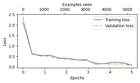
• Above, based on the downward slope, we see that the model learns well

• Furthermore, the fact that the training and validation loss are very close indicates that the model does not tend to overfit the training data

• Similarly, we can plot the accuracy below

epochs_tensor = torch.linspace(0, num_epochs, len(train_accs))
examples_seen_tensor = torch.linspace(0, examples_seen, len(train_accs))

plot_values(epochs_tensor, examples_seen_tensor, train_accs, val_accs, label="accuracy")

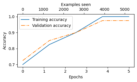
• Based on the accuracy plot above, we can see that the model achieves a relatively high training and validation accuracy after epochs 4 and 5

• However, we have to keep in mind that we specified eval_iter=5 in the training function earlier, which means that we only estimated the training and validation set performances

• We can compute the training, validation, and test set performances over the complete dataset as follows below

train_accuracy = calc_accuracy_loader(train_loader, model, device)
val_accuracy = calc_accuracy_loader(val_loader, model, device)
test_accuracy = calc_accuracy_loader(test_loader, model, device)

print(f"Training accuracy: {train_accuracy*100:.2f}%")
print(f"Validation accuracy: {val_accuracy*100:.2f}%")
print(f"Test accuracy: {test_accuracy*100:.2f}%")

Training accuracy: 97.21%
Validation accuracy: 97.32%
Test accuracy: 95.67%

• We can see that the training and test set performances are practically identical

• However, based on the slightly lower test set performance, we can see that the model overfits the training data to a very small degree

• This is normal, however, and this gap could potentially be further reduced by increasing the model’s dropout rate (drop_rate) or the weight_decay in the optimizer setting

7.8. Using the LLM as a spam classifier

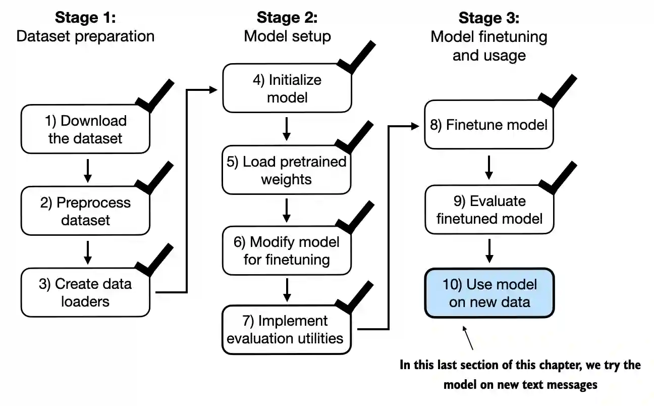
• Finally, let’s use the finetuned GPT model in action

• The classify_review function below implements the data preprocessing steps similar to the SpamDataset we implemented earlier

• Then, the function returns the predicted integer class label from the model and returns the corresponding class name

def classify_review(text, model, tokenizer, device, max_length=None, pad_token_id=50256):
    model.eval()

    # Prepare inputs to the model
    input_ids = tokenizer.encode(text)
    supported_context_length = model.pos_emb.weight.shape[1]

    # Truncate sequences if they too long
    input_ids = input_ids[:min(max_length, supported_context_length)]

    # Pad sequences to the longest sequence
    input_ids += [pad_token_id] * (max_length - len(input_ids))
    input_tensor = torch.tensor(input_ids, device=device).unsqueeze(0) # add batch dimension

    # Model inference
    with torch.no_grad():
        logits = model(input_tensor)[:, -1, :]  # Logits of the last output token
    predicted_label = torch.argmax(logits, dim=-1).item()

    # Return the classified result
    return "Positive" if predicted_label == 1 else "Negative"

• Let’s try it out on a few examples below

text_1 = (
    "You are a winner you have been specially"
    " selected to receive $1000 cash or a $2000 award."
)

print(classify_review(
    text_1, model, tokenizer, device, max_length=train_dataset.max_length
))

Positive

text_2 = (
    "Hey, just wanted to check if we're still on"
    " for dinner tonight? Let me know!"
)

print(classify_review(
    text_2, model, tokenizer, device, max_length=train_dataset.max_length
))

Negative

• Finally, let’s save the model in case we want to reuse the model later without having to train it again

torch.save(model.state_dict(), "review_classifier.pth")

• Then, in a new session, we could load the model as follows

model_state_dict = torch.load("review_classifier.pth")
model.load_state_dict(model_state_dict)

<All keys matched successfully>

7.9. Assignment

You can practice your cnn skills by following the assignment Fine-tuning Meta’s Llama 3 (8B) on your own data.